I recently worked through Udacity’s Data Engineering nanodegree program which consisted of four lessons:  Data Modeling (PostgreSQL and Cassandra) , Data Warehousing (Redshift), Data Lakes (Spark), and Pipeline Orchestration (Airflow).

In this post, I’ll share some of my notes from the second lesson: Data Warehousing. This lesson plan focused on deploying data warehouses on AWS using Redshift, so most of the discussion is specific to Redshift. Other cloud providers have similar Data Warehouse services, e.g. Google’s BigQuery.

What is a Data Warehouse?

The Data Warehouse is one of the central pillars of the Data Pipeline. In the last post, I talked about data modeling for OLTP databases like Relational databases running PostgreSQL and NoSQL databases running Cassandra. In this post, I’ll the core concepts behind OLAP (analytics) databases and some of the specifics of Redshift, AWS’s premiere Data Warehousing service. To get started, let’s revisit a diagram from an earlier post:

In this diagram, “Dimensional Model” is where the Data Warehouse sits. The process of ETL is performed by some code that is run on a schedule and meant to process data from the various transactions databases in batches and present the summarized data in a simpler schema. The simpler schema of the Data Warehouse is optimized for Ad-hoc queries by the analyst and BI teams. Data Warehouses are also used for archiving historical data, to lighten the resource requirements of the transactional databases.

You can think of the OLTP and OLAP databases as the “back of the house” and “front of the house” data stores. All the actual sales and operational processes are done in the back of the house with the OLTP (“T” is for transactional) databases, and then the results are brought up to the front of the house for visualization and analysis.

To reiterate a point from an earlier post, the point of having separate OLAP databases from your OLTP databases is that the OLTP databases are optimized for fast writes, not fast analytics. If you tried to do analytics on your transactions databases, it would just slow down your operations (and customers don’t like waiting a long time for their transactions to go through). So Data Warehouses are an infrastructure solution that fits in between Operations and Analytics which unloads data from the Operations side of things to the Analytical side of the business.

In the simplest ETL, our OLTP operations are executed on a 3NF database and the ETL just converts to a simpler Star Schema. OLTP does a lot of writes, and to optimize for writes, you want your schema to be as normalized as possible. This is where the basic database concepts of Facts and Dimensions comes into play when designing the Data Model.

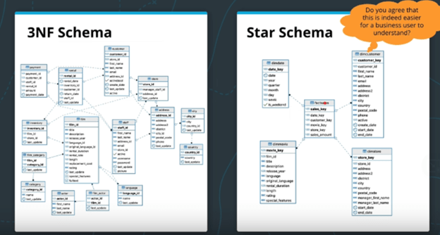
This is the diagram given by the course: The start schema is denormalized to some degree, but that makes it much easier for the business analytics teams to perform their tasks with the data with simpler queries and fewer JOINs. i.e. it makes ad-hoc queries easier to design.

Facts and Dimensions

Facts are like events. They are real things that have an impact on our database. They are the central focus of the Star Schema, the main entity that the data model is modeling.

Dimensions – These are people, products, and places that relate to the core Facts. These are pieces of information that we would like to store in the database. Each dimension table will have one or more Fact table that it can JOIN.

Sometime the database schema on the left in the image above is described as a Snowflake Schema. The schemas are highly normalized and may track data around multiple entities of interest. The Star Schema is therefore a denormalized version of the Snowflake Schema that is intended to focus on a single (or a small number of) Fact table.

Data Cubes

Along with the Star Schema for Data Warehouses, another import concept is the OLAP cube of Data Cube.

What is a data cube? Well, to be honest, Data Cubes are a bit of a misnomer. The core feature of the data cube is that they store aggregated data from the Star Schema. For example, in the image below, the data cube has three dimensions and stores the total revenue of ticket sales to various movies by city and month. The three dimensions of this data cube are movie, month, and city. But Data cubes aren’t limited to three dimensions. A seven-dimensional data cube is perfectly valid. The point of presenting a data in a data cube is that it breaks apart a key business metric (such as revenue) along multiple dimensions. Once data is in this storage method, it’s easy for analysts to rolling up, drilling down, slice and dice the data.

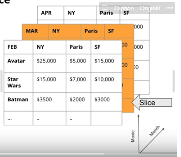
Data Cubes are typically stored in Relational Databases. They are so common that SQL supports a CUBE() operation. For example, the data in the image above might have be generated by a SQL statement similar to SELECT sum(sales) as Revenue FROM {tables} GROUP BY CUBE(movie, branch, month). This CUBE() operation will make one pass through the facts table and will aggregate all possible combinations of groupings of length 0, 1, 2, and 3.

The number of dimensions of a data cube is determined by the number of features that are included in the GROUP BY clause. For example, a data cube can be generated without the CUBE() operation by using the grouping sets operation. This effectively runs multiple queries in a single pass through the database and returns the result in a single output table:

SELECT month, country, sum(sales) as revenue
FROM factSales
JOIN DATE ON (Date.date_key = factSales.date_key)
JOIN Stores ON (Stores.store_key = Sales.store_key)
GROUP BY grouping sets ((), month, country, (month,country));

This runs four queries because the grouping sets clause has four positions. The first position () is like running the query without a GROUP BY clause (i.e. just return the total sum of all the sales). The second position groups by month, the third groups by country, and the fourth groups by both month and country. In this example, the dimension of the data cube that will be returned is 2 because you the biggest grouping set has two features: (month, country).

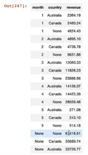
Below is the output of the above query. Notice the None in the results.  When you GROUP BY (), you will get None for both the month and the country columns because this is just the total revenue regardless of country or month. When None is in the month column, that’s GROUP BY country, and vise versa for GROUP BY month. Finally, each row that have both a value for month and country are the values were returned in response to GROUP BY (month, country). These values are essentially sub-totals of the overall revenue total calculated by GROUP BY ().

This is the same behavior that the in-built function CUBE() does. The following code returns the same output, with totals, sub-totals, and sub-sub-totals:

SELECT month, country, sum(sales) as revenue
FROM factSales
JOIN DATE ON (Date.date_key = factSales.date_key)
JOIN Stores ON (Stores.store_key = Sales.store_key)
GROUP BY CUBE(month,country);

Data Warehouses in the Cloud:

Data Warehouses are used for large amounts of data. When determining the required IT infrastructure, organizations have a branching decision tree of options. Between on-prem and cloud. Between self-managed cloud infrastructure and cloud-managed. Then between the various cloud services which have different hardware optimizations and trade-offs. The image below is taken from the Udacity course to illustrate the branching combination of choices when Architecting cloud infrastructure.

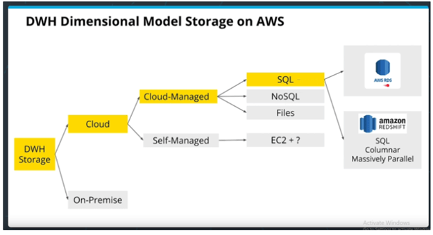
The benefit of self-managed is that it’s extremely customizable. If you need something very advanced or highly custom, then self-managed is the way to go. However, if commodity hardware is all you need, then Cloud-managed might be simpler and worth the extra cost.

This branching tree of options is why AWS has over 140 services, and why there are entire job titles for Cloud Solutions Architects. The amount of detailed knowledge that goes into creating these systems can be mind numbing for beginners. However, as I discussed in the first post in this series, most of the services on any cloud provider’s platform have parallel services on the other major platforms, so learning the details of one platform provides more valuable insight into the interplay of the various services than trying to learn the whole catalogue of services between all the platforms.

Data Warehouses on AWS:

RDS is a relational database “mixed managed” service. For the “fully managed” service, see Amazon Aurora. RDS instances can run any RDBMS software, including PostgreSQL. Aurora is “PostgreSQL-compatible” and is advertised to run three times faster than standard PostgreSQL databases. These systems are good for OLTP which is the backend of the data pipeline infrastructure.

Redshift is based on PostgreSQL and optimized for columnar storage and OLAP (analytics) processing. This is the king of AWS and what originally made AWS so good at Data Warehousing. It’s a “fully managed service” which means it auto-scales and has monitoring, software patching, failure recovery and auto-backups and all the rest. “Auto-scales” refers to the fact that Redshift is a distributed architecture and can therefore scale horizontally by adding more worker nodes to the network.

Redshift is also columnar storage, which is faster to retrieve and takes less space b/c of compression. RDS is row storage which is good for one-row read and writes (i.e. transactions). Amazon Redshift does not enforce primary key, foreign key and unique constraints, while RDS does. Amazon Redshift sorts the data before storing it in a table using the Sort Keys which enables faster retrieval. RDS obviously doesn’t do this.

Here is a good article on more of the difference between RDS (OLTP) and Redshift (OLAP): https://www.obstkel.com/amazon-redshift-vs-rds

Redshift and MPP database architectures:

As I just mentioned, Redshift has a distributed architecture. Most SQL RDBMS run single core operations on individual machines. This is useful if you have a high number of low computational queries because you can just make a queue for each core on the machine. (i.e. one query for one core.). This makes traditional Relational databases good for OLTP.

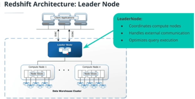
Redshift is what’s known as an MPP database (massively parallel processing) which parallelize the execution of queries on multiple cores/machines. Additionally, MPP is a distributed database architecture with distributed the data storage. So on top of MPP parallelizing individual queries on multiple cores, the query is being parallelized over multiple machines. The general architecture follows the typical architecture for distributed systems with a single Leader Node which commands multiple Compute Nodes. Each compute node is then further divided into “slices” which represent a single CPU with access to its own data storage.

Redshift lets you select the specs of the instances that make up your clusters. There are “Compute Optimized Nodes” and “Storage Optimized Nodes” where storage optimized basically just means it uses hard drives rather than SSDs or NVMe (which are much faster but more expensive for the same amount of memory).

Data partitioning of Redshift tables (Optimization of table design)

I just wanted to include a quick note on how Redshift distributes its data across multiple Node Slices. This is fairly similar to other distribute file storage systems, like Cassandra, but I skipped over this discussion in the previous post to have it here. Just note that this discussion of how to distributed and replicate data generally applies to many other distributed file systems.

However, remember that Cassandra did not allow JOINs between tables, while Redshift does.

Distribution Styles:

• EVEN distribution – the naive method. The data is randomly partitioned evenly between the number of CPUs (slices in compute nodes) in the network.
  • e.g. you are copying 1000 rows into Redshift, and you have 4 CPUs in your cluster, so 250 rows goes to each CPU. But this results in a lot of network traffic if you want to join two tables. JOINs result in lots of “shuffling” which means the CPUs must communicate with each other to determine what data they have to their local store.
• ALL distribution – small tables are copied to all CPUs, then the large tables are distributed evenly. This results in NO shuffling for joins involving small tables. Good! But this doesn’t solve the problem of large JOINs between two large tables.
• AUTO distribution – leaves the decision between ALL and EVEN to Redshift. Redshift uses a heuristic for determining what is “small enough” to be replicated to all CPUs.
• KEY distribution – Rows that have a similar value on a particular key column will all be put on the same CPU. Just like Cassandra’s Partition Key strategy. Redshift calls it distkey. This can result in an uneven distribution across CPU, though, if the distkey is skewed. Always choose a distribution key that is uniformly distributed by value.
• Sorting Key – Not used for partitioning but does help with optimization: If you have one column that is in the ORDER BY clause a lot, then setting the sort key can help optimize those queries. Note that you can set a column as both the distkey and sortkey.

In short, put the distkey on the big tables, and put them on a column that’s going to be uniformly distributed (like id or date). Then put the sortkey on any table on a column that will be order in the query result (like a rank, id, or date or datetime). And use diststyle all for all small tables. Note that if the data being copied into Redshift is already in the STAR schema, the dimension tables should be much smaller tables than the main fact table, and will be prime candidates for diststyle all.

Note that using these optimizations actually increases the time to create the table, but decreases query time, obviously. That’s not a problem for our OLAP database because many queries will be run on the table for every time new data is loaded to the database, so the trade-off is worth it. Here is a code example of the SQL required to create three tables in Redshift. Notice the use of sortkey, distkey, and diststyle all.

CREATE SCHEMA IF NOT EXISTS dist;
SET search_path TO dist;

DROP TABLE IF EXISTS part cascade;
DROP TABLE IF EXISTS supplier;
DROP TABLE IF EXISTS customer;

CREATE TABLE part (
  p_partkey     	integer     	not null	sortkey distkey,
  p_name        	varchar(22) 	not null,
  p_mfgr        	varchar(6)      not null,
  p_category    	varchar(7)      not null,
  p_brand1      	varchar(9)      not null,
  p_color       	varchar(11) 	not null,
  p_type        	varchar(25) 	not null,
  p_size        	integer     	not null,
  p_container   	varchar(10)     not null
);

CREATE TABLE supplier (
  s_suppkey     	integer        not null sortkey,
  s_name        	varchar(25)    not null,
  s_address     	varchar(25)    not null,
  s_city        	varchar(10)    not null,
  s_nation      	varchar(15)    not null,
  s_region      	varchar(12)    not null,
  s_phone       	varchar(15)    not null)
diststyle all;

CREATE TABLE customer (
  c_custkey     	integer        not null sortkey,
  c_name        	varchar(25)    not null,
  c_address     	varchar(25)    not null,
  c_city        	varchar(10)    not null,
  c_nation      	varchar(15)    not null,
  c_region      	varchar(12)    not null,
  c_phone       	varchar(15)    not null,
  c_mktsegment      varchar(10)    not null)
diststyle all;

Conclusion:

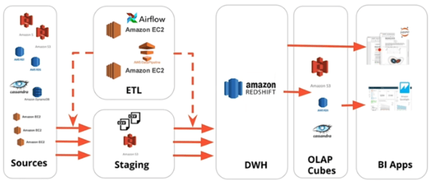
One final note about ETL pipelines and Data Warehouses. For whatever reason, it isn’t easy to get separate databases to communicate directly with each other. Instead, pipelines are typically designed to copy the results of a query to a file (either csv or json) on a staging instance or a cloud storage service. And then that file is copied to the Data Warehouse. On AWS, the whole pipeline might look something like this, where the code that operates the pipeline is run on the EC2 instances in the ETL block:

That’s the basics of Data Warehousing on AWS. It’s a large, distributed database designed for Big Data that is optimized for analysis and parallel processing of queries. The instructors of the course described MPP hardware as expensive, which they said gave rise to the next type of data storage: Data Lakes.