I recently worked through Udacity’s Data Engineering nanodegree program which consisted of four lessons:  Data Modeling (PostgreSQL and Cassandra), Data Warehousing (Redshift), Data Lakes (Spark), and Pipeline Orchestration (Airflow).

In this post, I’ll share some of my notes from the fourth and final lesson: Apache Airflow, which is an open-source pipeline orchestration software package and not specific to any particular cloud platform.

What is Airflow?

Apache Airflow was originally created by Airbnb and now has been released and adopted by the industry. It’s written in python and has one main job: schedule code to run automatically. The core concept of Apache Airflow is the DAG (Directed Acyclic Graph) which is a sequence of tasks that will be executed in order. Each task is a standalone process and can be a python function, SQL script, bash script, etc. In an ETL pipeline, the extract, transform, and load processes would each be their own task, and the DAG is the ordered sequence of these tasks, i.e. Airflow makes sure the Transform task isn’t started until the Extract task has successfully terminated, etc.. Each DAG in Airflow is automated to a set schedule. DAGs can be designed to run once or repeated on any kind of fixed interval, e.g. once per day, three times per day, once per hour, every hour of every other Tuesday, etc.)

Airflow Architecture:

There are five main components to the Airflow architecture. Starting from the right side in the figure below, the Worker nodes are the virtual machines that actually execute the tasks. These nodes are given the task to execute by the Queue database, which holds the current state of all the running DAGs and Tasks. When the workers are done with a task, that information will be sent up this architecture to either send the next task according to the DAG or wait for the other prerequisite tasks to be completed. The Scheduler actually orchestrates the high-level execute of DAGs including handling the logic of prerequisites and initiating DAGs according to their planned schedule. The Scheduler is the brains of the operation. The DB stores the metadata for Airflow including credentials. And finally, Airflow provides a User Interface (UI) to monitor, trigger, and maintain the DAGs using the Web Server.

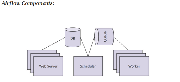
Note: Airflow workers are typically small computers. In an ELT pipeline with a Data Lake, the Airflow workers will trigger the Spark Cluster to perform the actual data processing.

DAGs

If you’re familiar with python, then Airflow will be very easy to pick up. DAGs are defined in a DAG file which is simply a python script with the suffix “_dag.py”. This DAG file will import the DAG class from the airflow library to instantiate a new DAG. There are two required arguments to instantiate a DAG: the name of the DAG, and the start_date. The name is a string with no spaces (e.g. ‘this.is.a.name’) and the start_date is a datetime object that is typically set to “today”. If the time is set to a specific date in the past, the Scheduler with repeat the DAG for the number of schedule_intervals between the start_date and today. This is used for processing a backlog, but it is not part of normal operations.

A few of the optional DAG arguments include:

• DAG description (string)
• schedule_interval (string) (default is ‘@daily’)
  •  ‘@once’ – Run a DAG once and then never again
  • ‘@hourly’ – Run the DAG every hour
  • ‘@daily’ – Run the DAG every day
  • ‘@weekly’ – Run the DAG every week
  • ‘@monthly’ – Run the DAG every month
  • ‘@yearly’ – Run the DAG every year
  • None – Only run the DAG when the User initiates it from the UI
  • Airflow also takes Cron Job schedule which take 5 positional arguments (6th is optional): min(0-59), hour(0-23), day of month (1-31), month (1-12), day of week (1-7, Sunday=7), year(optional)
    • e.g. ‘0 0 * * *’ will run every day at midnight.
• Retries (int) – the number of times a task will be retried before the DAG fails
• Retry_delay (timedelta) – the wait time between a task failing and the retry of the task

Once the DAG object is instantiated, tasks can be defined and assigned to the DAG. Each task is defined using an Operator function with have three required arguments: task_id (string), callable (the script or function that is called), and the dag (the DAG object that that was instantiated at the beginning of the file). At the beginning of this discussion, I mentioned that Airflow Tasks could be python functions, bash scripts, SQL operations, etc. Each type of Task requires a different type of Operator function to be called. For example, a python task requires the PythonOperator, while an SQL script might use the PostgresOperator.

There are many types of Airflow operators for every possible Task:

• PythonOperator
• PostgresOperator
• RedshiftToS3Operator
• S3ToRedshiftOperator
• BashOperator
• SimpleHttpOperator
• Sensor
• Etc.

You can also define custom operators or import custom libraries of operators. In each case, to use the operator, pass a script or a function that the operator will be able to execute to the callable parameter. Here is a toy example of what a basic DAG file might look like:

import datetime

from airflow import DAG
from airflow.operators.python_operator import PythonOperator

# define the python functions 

def say_hello(name):
    print(f"hello, {name}") 

def say_goodbye(name):
    print(f"goodbye, {name}") 

# Create the Airflow DAG object 

my_dag = DAG('name_that_dag',start_date=datetime.datetime.now(),schedule_interval='0 0 * * *') 

# Turn the functions to tasks 

start_pipeline = PythonOperator(
    task_id='the_task_name_is_say_hello',
    python_callable=say_hello,
    op_kwargs={'name'='Stephen'},
    dag=my_dag)

end_pipeline = PythonOperator(
    task_id='the_task_name_is_say_goodbye',
    python_callable=say_goodbye,
    op_kwargs={'name'='Stephen'},
    dag=my_dag)

# order the prerequisites 
start_pipeline >> end_pipeline

The code above specifies that the ‘name_that_dag’ DAG will be executed every day at midnight (the 0^th minute of the 0^th hour of every day). This DAG has two task: start_pipeline and end_pipeline, each of which take one argument: name. In each case, the name is passed to the task through the op_kwargs parameter.

There are other ways to pass parameters to a Task. For example, with “provide_context=True’, Airflow will pass a set of predefined context variables through the **kwargs parameter. See the Airflow documentation to see the list of default context variables. Here’s one example (Notice that the default context variables are passed to the hello_date task.):

from airflow import DAG
from airflow.operators.python_operator import PythonOperator

def hello_date(*args, **kwargs):
		print(f“Hello {kwargs[‘ds’]}”)    
		print(f“Hello {kwargs[‘execution_date’]}”)

divvy_dag = DAG(...)
task = PythonOperator(
    task_id=’hello_date’,
    python_callable=hello_date,
    provide_context=True,
    dag=divvy_dag)

Once the Tasks are defined according to the correct operator, the sequence of the tasks are defined using “>>”. For example:

op1 >> op2
op2 >> op4
op1 >> op3
op3 >> op4

Is the same as:

op1 >> op2 >> op4
op1 >> op3 >> op4

Is the same as:

op1 >> [op2, op3] >> op4

Each of the three examples above result in the same DAG. The first task, Op1, will be run when the DAG is triggered to run according to the interval_schedule. Upon completion of Op1, Op2 and Op3 will both be started. The Scheduler will waiter until both Op2 and Op3 are done before adding Op4 to the Queue. If one task executes before the other, the scheduler will wait for the other to be completed. Once Op4 executes successfully, the DAG is completed and will wait until it’s next scheduled interval to start again.

Additional notes on Airflow:

• “Small dags fail more gracefully”. For this reason, it’s a good practice to not build dags too large with too many dependencies. Separating large DAGs into multiple smaller DAGs also puts them on separate workers and can speed up processing time for the pipeline.  
• You can create multiple dags even within the same DAG file by instantiating multiple DAG objects with different names. It’s up to the designer of the pipeline whether to have multiple DAGs or a single DAG with has multiple parallel Tasks in it.
• Scheduling frequency is another consideration when determining the scale of your pipeline. But of course, the frequency is often set by the analysis that is needed rather than the data constraints.
• Tasks should be atomic. They should do one thing. If you can split them up, do it. Creating task boundaries is a best practice for building pipelines. In particular, “analyze” tasks are prime candidates to be atomized.
• Atomic tasks also make debugging errors much easier. Atomic tasks can also be parallelized which speeds up processing time. And they make the DAG more transparent (having a Task with a good, descriptive name is essential).

Monitoring options: Logs, GUI, SLA’s, email alters, and statsd (metrics tracking)

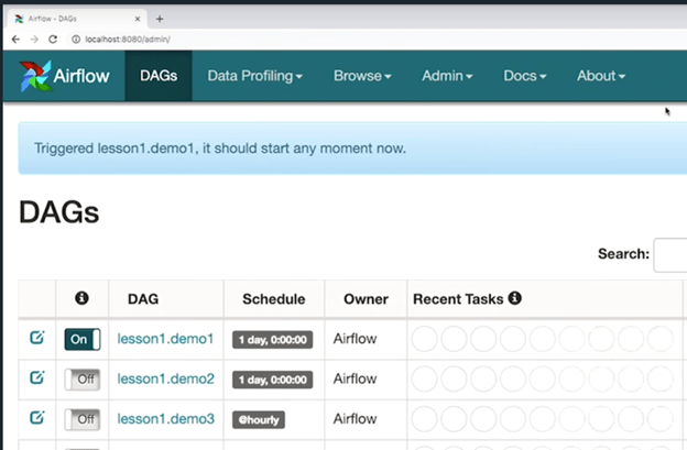
As I mentioned before, the Airflow GUI can be used to monitor the DAGs in the pipeline. The GUI will show active DAGs, the current task, the last time the DAG was executed, and the current state of the task (whether it has failed, how many times it’s failed, whether it’s currently retrying a failed DAG, etc.). DAGs can be trigger manually from the GUI as well as canceled. DAGs can also be “turned off” and removed from the schedule.

Service-Lev-Agreements (SLA) can be set from the GUI which will log when a pipeline fails or takes too long to execute. You can also set up email and slack alters to monitor your DAGs.

Additional Resources and References:

Examples of pipeline frameworks and libraries: https://github.com/pditommaso/awesome-pipeline

Airflow Contrib library (all the default operators): https://github.com/apache/airflow/tree/main/airflow/contrib

Comparing workflow scheduling frameworks: https://xunnanxu.github.io/2018/04/13/Workflow-Processing-Engine-Overview-2018-Airflow-vs-Azkaban-vs-Conductor-vs-Oozie-vs-Amazon-Step-Functions/

Conclusion:

That concludes this brief introduction to Airflow, as well as the final post on my notes from Udacity’s Data Engineering nanodegree program. Looking back, the four sections essentially covered four types of data storage systems: Relational Databases, NoSQL databases, Data Warehouses in the cloud, and Data Lakes in the cloud. The main technologies that were covered for each of these were PostgreSQL, Cassandra, AWS Redshift, and AWS EMR + Spark + HDFS, respectively. To be comprehensive, we might add AWS S3 buckets to this list of data stores, however, S3 is the only one in this list that doesn’t have any compute power associated with it (it’s just for storage).

The diversity of tools for data engineering underscores what some have been describing as the silver-bullet syndrome in which data engineers clamor for the latest and greatest tool stack available for Big Data only to find out that it doesn’t solve all of the challenges of Big Data and revert to the older technologies. A similar phenomenon is often observed with deep learning architectures despite many experienced deep learning practitioners suggesting the biggest gain in model performance can be observed with better data collection and processing rather than improvements in architecture.

The solution to the silver-bullet syndrome is, of course, to gain a firm grasp of the underlying principles and core concepts associated with each technology. For example, it’s striking to note that each of the four main data storage systems profiled in this online course operate on an SQL-like language. Even Data Lakes with Spark, which has Machine Learning libraries built into it, had SQL capabilities as the main driver of ETL operations. Despite SQL being over 50 years old (link to the original SQL paper, here), it’s still one of the primary technologies for manipulating data. The take-away is clear: To understand data pipelines, first understand SQL.

This course also discussed various concepts in distributed data storage and computation. It covered the CAP Theorem and the limitations it places on distributed storage systems. It covered distributed file systems like HDFS and cloud storage like AWS’s S3. And it covered the the core concepts of the MapReduce algorithm which powers the distributed computation of Data Lake tools like Apache Spark.

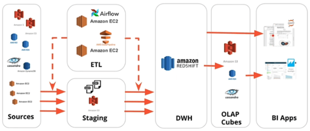
As a final review, I’ve included a diagram below from the course that I’ve shared before that shows the AWS services in their relative positions in a sample ETL pipeline. The only service missing from this diagram is the Data Lake which would consist of an EMR cluster running Spark (and potentially HDFS) and would be a middle-man between the EC2 instance running Airflow and the dotted lines pushing data from Source to Staging to DWH.

And that’s it. Those were the bulk of my notes from the nanodegree (minus all the code samples and exercises). The course itself obviously goes into greater detail than these notes and while it is a big unorganized at times, I’d recommend it to any software engineer who wants an introduction to the different types of databases. This course also serves as a useful introduction to Data Pipelines to anyone beginning their career in Data Engineering.